Joining Demographic Statistics onto a Dataset of Charity Donors with Python

Python

An anonymised display of voluntary work conducted for Emmanuel House Support Centre. Post 5/5 in the series.

Author

Daniel J Smith

Published

April 8, 2024

import numpy as np
import pandas as pd
import matplotlib.pyplot as plt
import seaborn as sns
import folium
from branca.colormap import LinearColormap
from sklearn.impute import KNNImputer

This post uses the dataset FakeIndividualConstituents.csv, comprising of 100 randomly selected postcodes in Nottingham city and crudely constructed donation behaviours for the ficticious donors these postcodes represent.

For the details of the construction of FakeIndividualConstituents.csv see a previous blog post.

This post follows some of my voluntary data analysis when studying a real dataset of donors to Emmanuel House in Nottingham.

df = pd.read_csv('files/FakeIndividualConstituents.csv')

df.head()

	Postcode	NumberDonations	TotalDonated	AverageDonated	Newsletter
0	NG9 3WF	4	61	15.25	1
1	NG9 4WP	1	23	23.00	0
2	NG9 3EL	1	30	30.00	0
3	NG1 9FH	5	75	15.00	1
4	NG5 6QZ	1	15	15.00	0

df.describe()

	NumberDonations	TotalDonated	AverageDonated	Newsletter
count	100.000000	100.000000	100.00000	100.000000
mean	4.320000	250.150000	46.51950	0.500000
std	5.454828	1657.135245	212.23961	0.502519
min	1.000000	15.000000	15.00000	0.000000
25%	1.000000	30.000000	15.00000	0.000000
50%	2.000000	45.000000	15.19000	0.500000
75%	5.000000	92.000000	16.92500	1.000000
max	37.000000	16618.000000	2077.25000	1.000000

GEOCODING

Lookup table connecting postcodes to the latitude/longitudes of their centres:

https://www.data.gov.uk/…

See previous blog posts (1) (2) for the details of this geocoding process.

post = pd.read_csv('LOOKUP_GEO/open_postcode_geo.csv', header=None, index_col=0)[[7, 8]]
post = post.rename(columns={7: 'Latitude', 8: 'Longitude'})
post.sample(5)

	Latitude	Longitude
0
EX19 8LW	50.916600	-4.060088
ML1 3LD	55.793773	-4.003318
NG17 8HS	53.112673	-1.268852
NG10 5AU	52.923366	-1.285042
WA1 3SS	53.399555	-2.570520

# Join Latitude and Longitude onto `df` using the 'Postcode' column
df = pd.merge(df, post, left_on='Postcode', right_index=True, how='left')

# Reorder the columns
df = df[['Postcode', 'Latitude', 'Longitude'] + [col for col in df.columns if col not in ['Postcode', 'Latitude', 'Longitude']]]

# Convert `Latitude` and `Longitude` columns from strings to floats
df['Latitude'] = pd.to_numeric(df['Latitude'], errors='coerce')
df['Longitude'] = pd.to_numeric(df['Longitude'], errors='coerce')

# Display number of null values in each column
df.isna().sum()

Postcode           0
Latitude           0
Longitude          0
NumberDonations    0
TotalDonated       0
AverageDonated     0
Newsletter         0
dtype: int64

df.head()

	Postcode	Latitude	Longitude	NumberDonations	TotalDonated	AverageDonated	Newsletter
0	NG9 3WF	52.930121	-1.198353	4	61	15.25	1
1	NG9 4WP	52.921587	-1.247504	1	23	23.00	0
2	NG9 3EL	52.938985	-1.239510	1	30	30.00	0
3	NG1 9FH	52.955008	-1.141045	5	75	15.00	1
4	NG5 6QZ	52.996670	-1.106307	1	15	15.00	0

JOINING OAs

In order to join demographic statistics onto the dataframe, we first need to convert postcodes into various output areas (OAs). Specifically OA2021, LSOA2021, LSOA2011 and MSOA2011.

What are Output Areas (OAs)?

Output Areas (OAs) are the smallest geographical unit for which census data is reported. In the UK, they were introduced for the 2001 Census and have been used since. They are designed to be of a similar population size, with each one containing at least 40 households and 100 individuals where possible. The aim is to provide a consistent base for reporting statistics over time.

Postcodes are a common way to identify locations in the UK, but they aren’t designed for statistical analysis. They can vary in size and can change over time. On the other hand, Output Areas are specifically designed for statistical analysis and are more stable over time.

By translating postcodes into Output Areas, we can join our postcode-level data with other datasets that use Output Areas.

JOINING LSOA2021 and OA2021 ONTO POSTCODE

Lookup table for converting Postcode to LSOA2021 and OA2021:

https://geoportal.statistics.gov.uk/…

# Read the lookup table and display 5 random rows
data = pd.read_csv('LOOKUP_GEO/PCD_OA21_LSOA21_MSOA21_LTLA22_UTLA22_CAUTH22_NOV23_UK_LU_v2.csv', low_memory=False)
data.sample(5)

	pcd7	pcd8	pcds	dointr	doterm	usertype	oa21cd	lsoa21cd	lsoa21nm	msoa21cd	msoa21nm	ltla22cd	ltla22nm	ltla22nmw	utla22cd	utla22nm	utla22nmw	cauth22cd	cauth22nm
2411384	TN4 0JY	TN4 0JY	TN4 0JY	198001	NaN	0	E00126111	E01024846	Tunbridge Wells 002C	E02005163	Tunbridge Wells 002	E07000116	Tunbridge Wells	NaN	E10000016	Kent	NaN	NaN	NaN
238683	BN3 7WA	BN3 7WA	BN3 7WA	200012	200212.0	1	E00085160	E01016873	Brighton and Hove 019D	E02003509	Brighton and Hove 019	E06000043	Brighton and Hove	NaN	E06000043	Brighton and Hove	NaN	NaN	NaN
1484466	ML3 6PJ	ML3 6PJ	ML3 6PJ	198001	NaN	0	S00131878	S01012725	NaN	S02002385	NaN	S12000029	South Lanarkshire	NaN	S12000029	South Lanarkshire	NaN	NaN	NaN
2320876	SW1X8DL	SW1X 8DL	SW1X 8DL	198001	NaN	0	E00190381	E01004691	Westminster 019E	E02000978	Westminster 019	E09000033	Westminster	NaN	E09000033	Westminster	NaN	NaN	NaN
2516422	W1J 5LF	W1J 5LF	W1J 5LF	200012	NaN	0	E00024109	E01004761	Westminster 018D	E02000977	Westminster 018	E09000033	Westminster	NaN	E09000033	Westminster	NaN	NaN	NaN

# Take and rename only the relevant columns ('pcds', 'oa21cd', 'lsoa21cd') of lookup table `data`
data = data[['pcds','oa21cd','lsoa21cd']].rename({'pcds':'Postcode', 
                                                  'oa21cd':'OA21', 
                                                  'lsoa21cd':'LSOA21'}, axis=1)

# Display 5 randomly chosen rows of lookup table
data.sample(5)

	Postcode	OA21	LSOA21
1217999	L37 3JL	E00035430	E01006990
2198583	SO1 3GD	E00086950	E01017216
123853	BA2 5JZ	E00072680	E01014389
206780	BL4 9RE	E00024606	E01004861
149180	BB7 9YF	E00128667	E01025351

# Joining 'OA21' and 'LSOA21' from the lookup table `data` onto donors `df` using the 'Postcode' column
df = df.merge(data, on='Postcode', how='left')

# Display number of null values in each column to see if successful
df.isna().sum()

Postcode           0
Latitude           0
Longitude          0
NumberDonations    0
TotalDonated       0
AverageDonated     0
Newsletter         0
OA21               0
LSOA21             0
dtype: int64

df.sample(5)

	Postcode	Latitude	Longitude	NumberDonations	TotalDonated	AverageDonated	Newsletter	OA21	LSOA21
72	NG2 7DL	52.945107	-1.135586	1	16	16.00	0	E00173532	E01033402
39	NG8 9QN	52.959883	-1.222125	9	138	15.33	1	E00069921	E01013860
37	NG8 3DJ	52.970564	-1.219671	4	60	15.00	1	E00069940	E01013867
97	NG9 2QA	52.930121	-1.198353	1	15	15.00	0	E00187586	E01028074
59	NG11 7AX	52.925360	-1.157251	1	539	539.00	1	E00070145	E01013901

JOINING MSOA2011 ONTO POSTCODE

Lookup table for converting Postcode to MSOA2011:

https://geoportal.statistics.gov.uk/…

Please note that I have renamed my file to pcd_to_oa11_msoa11_lsoa11.csv from PCD_OA_LSOA_MSOA_LAD_MAY22_UK_LU.csv which was the name it had at download time.

# Read the lookup table and display 5 randomly chosen rows
data = pd.read_csv('LOOKUP_GEO/pcd_to_oa11_msoa11_lsoa11.csv', encoding='ISO-8859-1', low_memory=False)
data.sample(5)

	pcd7	pcd8	pcds	dointr	doterm	usertype	oa11cd	lsoa11cd	msoa11cd	ladcd	lsoa11nm	msoa11nm	ladnm	ladnmw
359020	BT8 6ZS	BT8 6ZS	BT8 6ZS	200912	NaN	0	N00001771	95II03S1	N99999999	N09000007	Cairnshill 1	(pseudo) Northern Ireland	Lisburn and Castlereagh	NaN
1700528	NW8 9QR	NW8 9QR	NW8 9QR	198001	NaN	0	E00023413	E01004648	E02000961	E09000033	Westminster 002B	Westminster 002	Westminster	NaN
945738	GL6 8WR	GL6 8WR	GL6 8WR	200212	200904.0	1	E00113923	E01022411	E02004656	E07000082	Stroud 006D	Stroud 006	Stroud	NaN
1056104	HU120NG	HU12 0NG	HU12 0NG	198001	NaN	0	E00066007	E01013079	E02002722	E06000011	East Riding of Yorkshire 039A	East Riding of Yorkshire 039	East Riding of Yorkshire	NaN
267517	BS161UY	BS16 1UY	BS16 1UY	201808	NaN	0	E00173035	E01033333	E02003106	E06000025	South Gloucestershire 017F	South Gloucestershire 017	South Gloucestershire	NaN

# Take and rename only the relevant columns ('pcds', 'msoa11cd') of lookup table `data`
data = data[['pcds', 'msoa11cd']].rename({'pcds':'Postcode',
                                          'msoa11cd':'MSOA11'}, axis=1)

# Display 5 randomly chosen rows
data.sample(5)

	Postcode	MSOA11
2292291	SW18 1BW	E02000932
939836	GL52 4JT	E02004670
2630775	WV12 5TE	E02002123
2617558	WS13 6TL	E02006150
663239	DH7 9RF	E02004307

# Joining 'MSOA11' from the lookup table `data` onto donors `df` using the 'Postcode' column:
df = df.merge(data, on='Postcode', how='left')
 
# Display number of null values in each column to see if successful:
df.isna().sum()

Postcode           0
Latitude           0
Longitude          0
NumberDonations    0
TotalDonated       0
AverageDonated     0
Newsletter         0
OA21               0
LSOA21             0
MSOA11             1
dtype: int64

JOINING DEMOGRAPHIC STATISTICS ONTO OAs

Understanding the Index of Multiple Deprivation (IMD) Score

The IMD Score is a measure of relative deprivation for small areas in the UK. It combines information from seven domains to produce an overall relative measure of deprivation. The higher the IMD Score, the more deprived an area is considered to be. Unlike the IMD Rank, which ranks areas in order, the IMD Score provides a measure of the absolute level of deprivation.

Joining IMD2019 onto `df` by first coverting LSOA2021 to LSOA2011:

Lookup table coverting LSOA2021 to LSOA2011:

https://geoportal.statistics.gov.uk/…

Lookup table converting LSOA2011 to Index of Multiple Deprivation (IMD) 2019:

https://www.gov.uk/government/statistics/…

# Read the LSOA lookup data
lookup_data = pd.read_csv('LOOKUP_GEO/LSOA_(2011)_to_LSOA_(2021)_to_Local_Authority_District_(2022)_Lookup_for_England_and_Wales_(Version_2).csv')

# Take only the relevant columns of `lookup_data` and rename
lookup_data = lookup_data[['LSOA21CD','LSOA11CD']].rename({'LSOA21CD':'LSOA21', 
                                                           'LSOA11CD':'LSOA11'}, axis=1)

# Read the IMD data
imd_data = pd.read_csv('LOOKUP_STATS/File_7_-_All_IoD2019_Scores__Ranks__Deciles_and_Population_Denominators_3.csv')

# Take only the relevant columns of `imd_data` and rename
imd_data = imd_data[['LSOA code (2011)', 'Index of Multiple Deprivation (IMD) Score']].rename({'LSOA code (2011)':'LSOA11', 
                                                                                               'Index of Multiple Deprivation (IMD) Score':'IMD_Score'}, axis=1)

There is not a 1-to-1 correspondence between LSOA2011 and LSOA2021. We work around this by aggregating over the different LSOA2011 corresponding to each LSOA2021 and returning the mean of the IMD scores of each.

# Merge the IMD data with the lookup data
imd_data = imd_data.merge(lookup_data, on='LSOA11', how='left')

# Aggregate the IMD scores for each LSOA21 by taking the mean
imd_data = imd_data.groupby('LSOA21')['IMD_Score'].mean().reset_index()

# Joining 'IMD_Score' from the aggregated lookup table `imd_data` onto donors `df` using the 'LSOA21' column
df = df.merge(imd_data, on='LSOA21', how='left')

# Display number of null values in 'IMD_Score' column of `df` after the join
df['IMD_Score'].isna().sum()

Using `KNNImputer` to fill missing IMD scores:

# Create a new dataframe with only the columns of interest
geo_data = df[['Latitude', 'Longitude', 'IMD_Score']]

# Create the imputer
imputer = KNNImputer(n_neighbors=5, weights='distance')

# Apply the imputer to the geo_data
geo_data_filled = imputer.fit_transform(geo_data)

# Convert the result back to a dataframe and preserve the original index
geo_data_filled = pd.DataFrame(geo_data_filled, columns=geo_data.columns, index=geo_data.index)

# Replace the original 'IMD_Score' column with the 'IMD_Score' with missing values filled
df['IMD_Score'] = geo_data_filled['IMD_Score']

df['IMD_Score'].isna().sum()

Joining population density onto LSOA2021:

Lookup table connecting LSOA2021 to population density:

https://www.ons.gov.uk/peoplepopulationandcommunity/…

Please note I used the ‘Mid-2020: SAPE23DT11’ edition of this dataset.

# Read the lookup table and display 5 randomly chosen rows
Pop_density_lookup = pd.read_csv('LOOKUP_STATS/sape23dt11mid2020lsoapopulationdensity 4(Sheet1).csv')
Pop_density_lookup.sample(5)

	LSOA Code	LSOA Name	Mid-2020 population	Area Sq Km	People per Sq Km
17470	E01029204	South Somerset 009C	1,205	3.99	302
28309	E01000300	Barnet 019B	1,763	0.17	10,161
30690	E01002662	Hounslow 017C	2,658	0.24	10,862
23151	E01007102	Sefton 030D	1,516	0.20	7,535
29991	E01032790	Hammersmith and Fulham 023F	1,440	0.08	18,228

# Take and rename only the relevant columns ('LSOA Code', 'People per Sq Km') of lookup table `Pop_density_lookup`
Pop_density_lookup = Pop_density_lookup[['LSOA Code','People per Sq Km']].rename({'LSOA Code':'LSOA21', 
                                                                                  'People per Sq Km':'PopDensity'},axis=1)

# Display 5 randomly chosen rows
Pop_density_lookup.sample(5)

	LSOA21	PopDensity
18268	E01030319	1,476
10776	E01021912	194
1907	E01013840	6,024
15518	E01026885	55
7355	E01015276	9,177

# Joining 'PopDensity' from the lookup table `Pop_density_lookup` onto donors `df` using the 'LSOA21' column:
df = df.merge(Pop_density_lookup, on='LSOA21', how='left')

# Remove commas from joined population densities and convert to float type:
df['PopDensity'] = df['PopDensity'].str.replace(',', '').astype(float)

# Display number of null values in 'PopDensity' column:
df['PopDensity'].isna().sum()

Using `KNNImputer` to fill missing population densities

# Create a new dataframe with only the columns of interest
pop_data = df[['Latitude', 'Longitude', 'PopDensity']]

# Create the imputer
imputer = KNNImputer(n_neighbors=5, weights='distance')

# Apply the imputer to the `pop_data`
pop_data_filled = imputer.fit_transform(pop_data)

# Convert the result back to a dataframe and preserve the original index
pop_data_filled = pd.DataFrame(pop_data_filled, columns=pop_data.columns, index=pop_data.index)

# Replace original 'PopDensity' column with the 'PopDensity' column with missing values filled
df['PopDensity'] = pop_data_filled['PopDensity']

df['PopDensity'].isna().sum()

Joining Average Annual Income onto MSOA2011

Lookup table joining MSOA2011 to Average Annual Income:

https://www.ons.gov.uk/employmentandlabourmarket/…

Please note that my file MSOA2011_to_Income.csv is the ‘Total Annual Income’ sheet of the Financial year ending 2020 edition of this dataset.

# Read the lookup table and display 5 randomly chosen rows
income_lookup = pd.read_csv('LOOKUP_STATS/MSOA2011_to_Income.csv', encoding='ISO-8859-1', low_memory=False)
income_lookup.sample(5)

	MSOA code	MSOA name	Local authority code	Local authority name	Region code	Region name	Total annual income (£)	Upper confidence limit (£)	Lower confidence limit (£)	Confidence interval (£)
6820	W02000030	Conwy 004	W06000003	Conwy	W92000004	Wales	34,400	40,900	28,900	12,000
2082	E02006827	Amber Valley 017	E07000032	Amber Valley	E12000004	East Midla	35,500	42,100	29,800	12,300
6309	E02003135	Plymouth 014	E06000026	Plymouth	E12000009	South West	40,900	49,000	34,200	14,800
1074	E02005327	Wyre 009	E07000128	Wyre	E12000002	North West	42,300	50,000	35,700	14,300
4319	E02000880	Tower Hamlets 017	E09000030	Tower Hamlets	E12000007	London	50,500	59,800	42,600	17,200

# Take and rename only the relevant columns ('MSOA code', 'Total annual income (£)') of lookup table `income_lookup`
income_lookup = income_lookup[['MSOA code','Total annual income (£)']].rename({'MSOA code':'MSOA11', 
                                                                               'Total annual income (£)':'AvgAreaIncome'}, axis=1)

# Display 5 randomly chosen rows
income_lookup.sample(5)

	MSOA11	AvgAreaIncome
717	E02001117	46,900
2198	E02005364	42,500
4561	E02000195	59,500
6000	E02006543	45,500
3514	E02004466	51,700

# Joining 'AvgAreaIncome' from the lookup table `income_lookup` onto donors `df` using the 'MSOA11' column:
df = df.merge(income_lookup, on='MSOA11', how='left')

# Removing commas from incomes and converting to float type:
df['AvgAreaIncome'] = df['AvgAreaIncome'].str.replace(',', '').astype(float)

# Display number of null values in 'AvgAreaIncome' column:
df['AvgAreaIncome'].isna().sum()

Using `KNNImputer` to fill missing ‘AvgAreaIncome’ values

# Create a new dataframe `inc_data` with only the columns of interest
inc_data = df[['Latitude', 'Longitude', 'AvgAreaIncome']]

# Create the imputer
imputer = KNNImputer(n_neighbors=5, weights='distance')

# Apply the imputer to the `inc_data` dataframe
inc_data_filled = imputer.fit_transform(inc_data)

# Convert the result back to a dataframe and preserve the original index
inc_data_filled = pd.DataFrame(inc_data_filled, columns=inc_data.columns, index=inc_data.index)

# Replace original 'AvgAreaIncome' column with the corresponding column with missing values filled
df['AvgAreaIncome'] = inc_data_filled['AvgAreaIncome']

df['AvgAreaIncome'].isna().sum()

VISUALISING RESULTS WITH FOLIUM

m = folium.Map(location=[52.9548, -1.1581], zoom_start=12)

colors = ['green', 'yellow', 'orange', 'red', 'purple']
linear_colormap = LinearColormap(colors=colors,
                                 vmin=df['PopDensity'].min(),
                                 vmax=df['PopDensity'].quantile(0.9))


for index, row in df.iterrows():    
    num_don = row['NumberDonations']
    total_don = row['TotalDonated']
    news = bool(row['Newsletter'])
    avg_don = row['AverageDonated']

    imd = row['IMD_Score']
    inc = row['AvgAreaIncome']
    pop = row['PopDensity']
    
    # Add popups when a marker clicked on
    popup_text = f'''
                    <div style="width: 250px; font-family: Arial; line-height: 1.2;">
                        <h4> Donation History: </h4>
                        <p style="margin: 0;"><b>Total Donated:</b> £{total_don:.2f}</p>
                        <p style="margin: 0;"><b>Number of Donations:</b> {num_don}</p>
                        <p style="margin: 0;"><b>Average Donation:</b> £{avg_don:.2f}</p>
                        <p style="margin: 0;"><b>Subscribed to Newsletter:</b> {"Yes" if news else "No"}</p>
                        <br>

                        <h4> Local Demographic Statistics: </h4>
                        <p style="margin: 0;"><b>Local Population Density:</b> {pop:.2f} ppl/km2</p>
                        <p style="margin: 0;"><b>Local IMD Score:</b> {imd:.2f}</p>
                        <p style="margin: 0;"><b>Local Average Income:</b> £{inc:.2f}</p>
                    </div>
                    '''

    color = linear_colormap(pop)
    
    marker = folium.CircleMarker(
        location=[row['Latitude'], row['Longitude']],
        radius=5,
        color=color, 
        fill=True,
        fill_color=color,
        fill_opacity=1,
        popup=popup_text
    ).add_to(m)
    

linear_colormap.add_to(m)
linear_colormap.caption = 'Population Density (Ppl per Sq Km)'

m

Make this Notebook Trusted to load map: File -> Trust Notebook

In the above map, the markers for each donor are coloured by that donors local population density.

There is an clear trend of increasing population density as we move towards central Nottingham.

Relationships between demographic statistics & donation history

IMD Score

fig, axs = plt.subplots(1, 2, figsize=(24, 8))

# Total Donated vs IMD Score scatterplot
sns.scatterplot(x=df['IMD_Score'], y=df['TotalDonated'], ax=axs[0])
sns.regplot(x=df['IMD_Score'], y=df['TotalDonated'], scatter=False, color='red', ax=axs[0], ci=None)
corr = np.corrcoef(df['IMD_Score'], df['TotalDonated'])[0, 1]
axs[0].annotate(f'Correlation: {corr:.2f}', xy=(0.95, 0.95), xycoords='axes fraction',
                fontsize=12, ha='right', va='top', bbox=dict(boxstyle='round', fc='firebrick', alpha=0.5))
axs[0].set_ylim(0,1500)
axs[0].set_ylabel('Total Donated (£)')
axs[0].set_title('Lifetime Donation Total vs IMD Score')

# Number Donations vs IMD Score scatterplot
sns.scatterplot(x=df['IMD_Score'], y=df['NumberDonations'], ax=axs[1])
sns.regplot(x=df['IMD_Score'], y=df['NumberDonations'], scatter=False, color='red', ax=axs[1], ci=None)
corr = np.corrcoef(df['IMD_Score'], df['NumberDonations'])[0, 1]
axs[1].annotate(f'Correlation: {corr:.2f}', xy=(0.95, 0.95), xycoords='axes fraction',
                fontsize=12, ha='right', va='top', bbox=dict(boxstyle='round', fc='firebrick', alpha=0.5))
axs[1].set_ylabel('Number of Donations')
axs[1].set_title('Number of Donations vs IMD Score')

plt.show()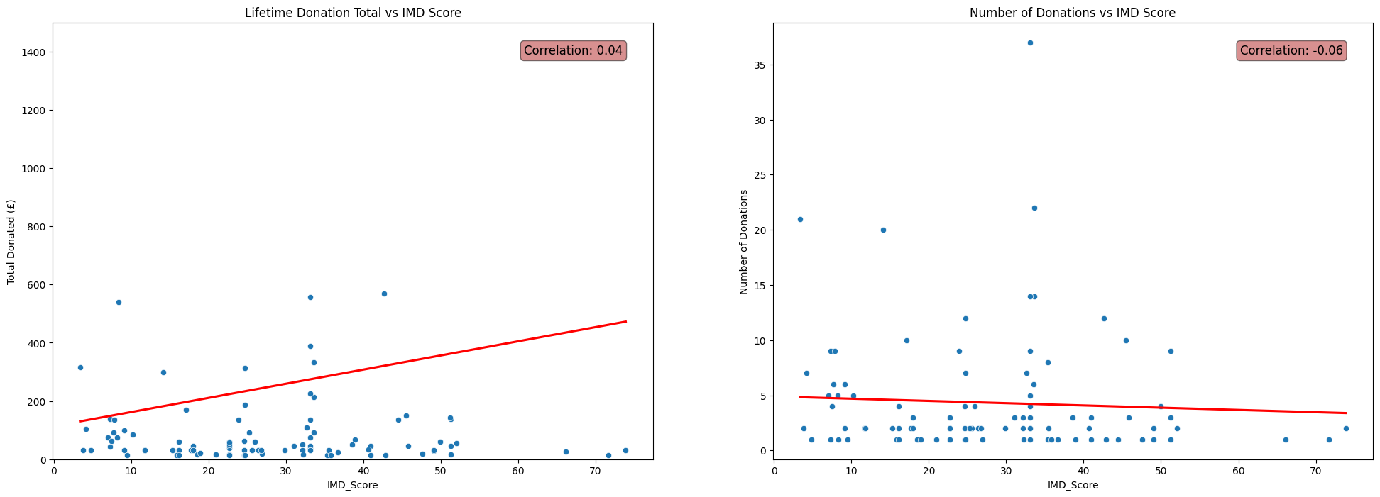

Population Density

fig, axs = plt.subplots(1, 2, figsize=(24, 8))

# Total Donated vs Population Density scatterplot
sns.scatterplot(x=df['PopDensity'], y=df['TotalDonated'], ax=axs[0])
sns.regplot(x=df['PopDensity'], y=df['TotalDonated'], scatter=False, color='red', ax=axs[0], ci=None)
corr = np.corrcoef(df['PopDensity'], df['TotalDonated'])[0, 1]
axs[0].annotate(f'Correlation: {corr:.2f}', xy=(0.95, 0.95), xycoords='axes fraction',
                fontsize=12, ha='right', va='top', bbox=dict(boxstyle='round', fc='firebrick', alpha=0.5))
axs[0].set_ylim(0,800)
axs[0].set_ylabel('Total Donated (£)')
axs[0].set_xlabel('Local Population Density (People per Sq Km)')
axs[0].set_title('Lifetime Donation Total vs Population Density')

# Number Donations vs Population Density scatterplot
sns.scatterplot(x=df['PopDensity'], y=df['NumberDonations'], ax=axs[1])
sns.regplot(x=df['PopDensity'], y=df['NumberDonations'], scatter=False, color='red', ax=axs[1], ci=None)
corr = np.corrcoef(df['PopDensity'], df['NumberDonations'])[0, 1]
axs[1].annotate(f'Correlation: {corr:.2f}', xy=(0.95, 0.95), xycoords='axes fraction',
                fontsize=12, ha='right', va='top', bbox=dict(boxstyle='round', fc='firebrick', alpha=0.5))
axs[1].set_ylim(0,30)
axs[1].set_ylabel('Number of Donations')
axs[1].set_xlabel('Local Population Density (People per Sq Km)')
axs[1].set_title('Number of Donations vs Population Density')

plt.show()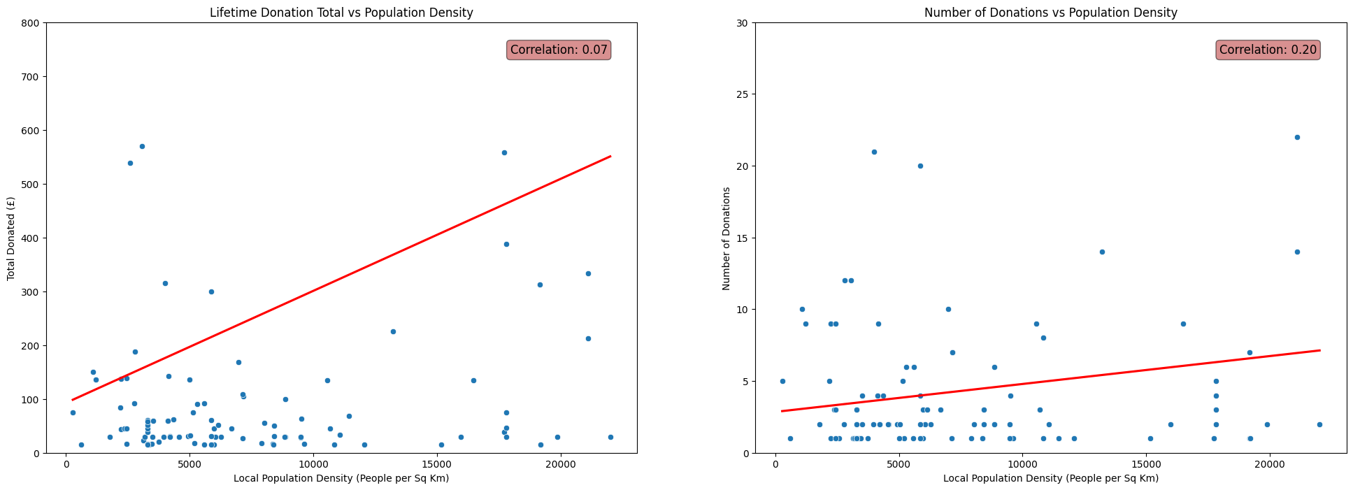

Average Income

fig, axs = plt.subplots(1, 2, figsize=(24, 8))

# Total Donated vs Average Income scatterplot
sns.scatterplot(x=df['AvgAreaIncome'], y=df['TotalDonated'], ax=axs[0])
sns.regplot(x=df['AvgAreaIncome'], y=df['TotalDonated'], scatter=False, color='red', ax=axs[0], ci=None)
corr = np.corrcoef(df['AvgAreaIncome'], df['TotalDonated'])[0, 1]
axs[0].annotate(f'Correlation: {corr:.2f}', xy=(0.95, 0.95), xycoords='axes fraction',
                fontsize=12, ha='right', va='top', bbox=dict(boxstyle='round', fc='firebrick', alpha=0.5))
axs[0].set_ylim(-200,2000)
axs[0].set_ylabel('Total Donated (£)')
axs[0].set_xlabel('Average Income (£)')
axs[0].set_title('Lifetime Donation Total vs Average Income')

# Number Donations vs Average Income scatterplot
sns.scatterplot(x=df['AvgAreaIncome'], y=df['NumberDonations'], ax=axs[1])
sns.regplot(x=df['AvgAreaIncome'], y=df['NumberDonations'], scatter=False, color='red', ax=axs[1], ci=None)
corr = np.corrcoef(df['AvgAreaIncome'], df['NumberDonations'])[0, 1]
axs[1].annotate(f'Correlation: {corr:.2f}', xy=(0.95, 0.95), xycoords='axes fraction',
                fontsize=12, ha='right', va='top', bbox=dict(boxstyle='round', fc='firebrick', alpha=0.5))
#axs[1].set_ylim(0,30)
axs[1].set_ylabel('Number of Donations')
axs[1].set_xlabel('Average Income (£)')
axs[1].set_title('Number of Donations vs Average Income')

plt.show()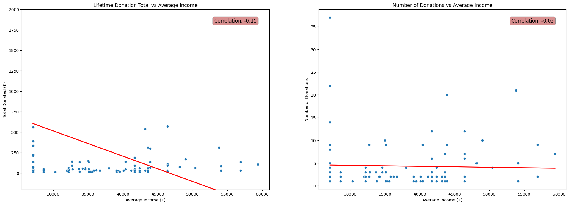

Remarks

It may be tempting to write off the negligble correlations shown in the above plots as facets of the fact that the donors in FakeIndividualConstituents.csv have randomly selected postcodes and crudely contructed donation histories.

(See my previous post for the details of the contruction of this dataset.)

This means we perhaps shouldn’t expect to see any non-negligible correlations, due to the random nature of the process used to produce the fake data that did not take into account properties like population density.

However, the patterns shown in the real data were very similar. In fact, the correlations between each of IMD Score, Population Density and Average Income with Number of Donations and Total Donated were even closer to zero for the dataset of real donors to Emmanuel House than for the fake dataset used above.

This initially suprised me. I thoroughly expected for the data to display a clear relationship between the social deprivation of the area in which donors live and their donation patterns. In reality this was not reflected in the data at all.

It may be that the relationship between these statistics and a donor’s behaviour is far more complicated than linear, and thus is not well described by the correlation coefficient.

On the other hand, it may be that there is no interpretable relationship between a donors demographic statistics and their donation behaviour.

GEOCODING

JOINING OAs

What are Output Areas (OAs)?

JOINING LSOA2021 and OA2021 ONTO POSTCODE

JOINING MSOA2011 ONTO POSTCODE

JOINING DEMOGRAPHIC STATISTICS ONTO OAs

Understanding the Index of Multiple Deprivation (IMD) Score

Joining IMD2019 onto df by first coverting LSOA2021 to LSOA2011:

Using KNNImputer to fill missing IMD scores:

Joining population density onto LSOA2021:

Using KNNImputer to fill missing population densities

Joining Average Annual Income onto MSOA2011

Using KNNImputer to fill missing ‘AvgAreaIncome’ values

VISUALISING RESULTS WITH FOLIUM

Relationships between demographic statistics & donation history

IMD Score

Population Density

Average Income

Remarks

Joining IMD2019 onto `df` by first coverting LSOA2021 to LSOA2011:

Using `KNNImputer` to fill missing IMD scores:

Using `KNNImputer` to fill missing population densities

Using `KNNImputer` to fill missing ‘AvgAreaIncome’ values